A gentle introduction to OCR
Intro
OCR, or optical character recognition, is one of the earliest addressed computer vision tasks, since in some aspects it does not require deep learning. Therefore there were different OCR implementations even before the deep learning boom in 2012, and some even dated back to 1914 (!).
This makes many people think the OCR challenge is “solved”, it is no longer challenging. Another belief which comes from similar sources is that OCR does not require deep learning, or in other words, using deep learning for OCR is an overkill.
Anyone who practices computer vision, or machine learning in general, knows that there is no such thing as a solved task, and this case is not different. On the contrary, OCR yields very-good results only on very specific use cases, but in general, it is still considered as challenging.
Additionally, it’s true there are good solutions for certain OCR tasks that do not require deep learning. However, to really step forward towards better, more general solutions, deep learning will be mandatory.
Why do I write about OCR?
As many of my works/write-ups, this too started off as project for client. I was requested to solve a specific OCR task.
During and after working on this task, I’ve reached some conclusions and insights which I was very eager to share with you. Additionally, after intensively working on such a task, it is hard for me to stop and throw it away, so I keep my research going, and hoping to achieve an even better and more generalized solution.
What you’ll find here
In this post I will explore some of the strategies, methods and logic used to address different OCR tasks, and will share some useful approaches. In the last part, we will tackle a real world problem with code. This should not be considered as an exhaustive review (unfortunately) since the depth, history and breadth of approaches are too wide for this kind of a blog-post.
However, as always, I will not spare you from references to articles, data sets, repositories and other relevant blog-posts.
Types of OCR
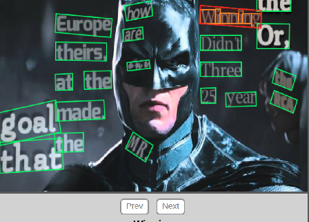
As I hinted before, there are more than one meaning for OCR. In its most general meaning, it refers to extracting text from every possible image, be it a standard printed page from a book, or a random image with graffiti in it (“in the wild”). In between, you may find many other tasks, such as reading license plates, no-robot captchas, street signs etc.
Although each of these options has its own difficulties, clearly “in the wild” task is the hardest.
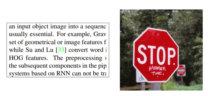
Form these examples we can draw out some attributes of the OCR tasks:
- Text density: on a printed/written page, text is dense. However, given an image of a street with a single street sign, text is sparse.
- Structure of text: text on a page is structured, mostly in strict rows, while text in the wild may be sprinkled everywhere, in different rotations.
- Fonts: printed fonts are easier, since they are more structured then the noisy hand-written characters.
- Character type: text may come in different language which may be very different from each other. Additionally, structure of text may be different from numbers, such as house numbers etc.
- Artifacts: clearly, outdoor pictures are much noisier than the comfortable scanner.
- Location: some tasks include cropped/centered text, while in others, text may be located in random locations in the image.
Data sets/Tasks
SVHN
A good place to start from is SVHN, Street View House Numbers data-set. As its name implies, this is a data-set of house numbers extracted from google street view. The task difficulty is intermediate. The digits come in various shapes and writing styles, however, each house number is located in the middle of the image, thus detection is not required. The images are not of a very high resolution, and their arrangement may be a bit peculiar.
License plates
Another common challenge, which is not very hard and useful in practice, is the license plate recognition. This task, as most OCR tasks, requires to detect the license plate, and then recognizing it’s characters. Since the plate’s shape is relatively constant, some approach use simple reshaping method before actually recognizing the digits. Here are some examples from the web:

- OpenALPR is a very robust tool, with no deep learning involved, to recognize license plates from various countries
- This repo provides an implementation of CRNN model (will be further discussed) to recognize Korean license plates.
- Supervise.ly, a data utilities company, wrote about training a license plate recognizer using artificial data generated by their tool (artificial data will also be further discussed)
CAPTCHA
Since the internet is full of robots, a common practice to tell them apart from real humans, are vision tasks, specifically text reading, aka CAPTCHA. Many of these texts are random and distorted, which should make it harder for computer to read. I’m not sure whoever developed the CAPTCHA predicted the advances in computer vision, however most of today text CAPTCHAs are not very hard to solve, especially if we don’t try to solve all of them at once.

Adam Geitgey provides a nice tutorial to solving some CAPTCHAs with deep learning, which includes synthesizing artificial data once again.
PDF OCR
The most common scenario for OCR is the printed/pdf OCR. The structured nature of printed documents make it much easier to parse them. Most OCR tools (e.g Tesseract) are mostly intended to address this task, and achieve good result. Therefore, I will not elaborate too much on this task in this post.
OCR in the wild
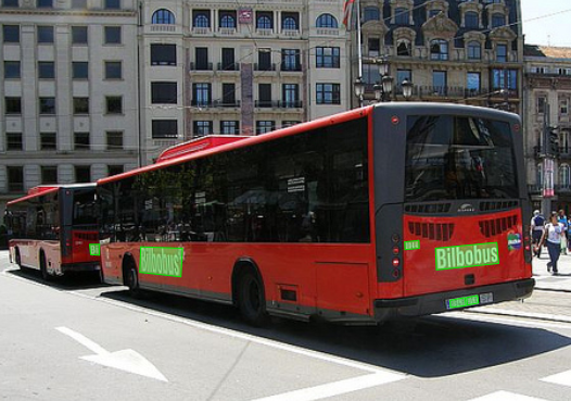
This is the most challenging OCR task, as it introduces all general computer vision challenges such as noise, lighting, and artifacts into OCR. Some relevant data-sets for this task is the coco-text, and the SVT data set which once again, uses street view images to extract text from.
Synth text
SynthText is not a data-set, and perhaps not even a task, but a nice idea to improve training efficiency is artificial data generation. Throwing random characters or words on an image will seem much more natural than any other object, because of the flat nature of text.
We have seen earlier some data generation for easier tasks like CAPTCHA and license plate. Generating text in the wild is a little bit more complex. The task includes considering depth information of an image. Fortunately, SynthText is a nice work that takes in images with the aforementioned annotations, and intelligently sprinkles words (from newsgroup data-set).
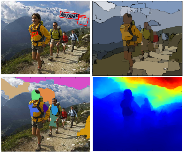
To make the “sprinkled” text look realistic and useful, the SynthText library takes with every image two masks, one of depth and another of segmentation. If you like to use your own images, you should add this data as well
- It is recommended to check the repo and generate some images on your own. You should pay attention that the repo uses some outdated version of opencv and maptlotlib, so some modifications may be necessary.
Mnist
Although not really an OCR task, it is impossible to write about OCR and not include the Mnist example. The most well known computer vision challenge is not really an considered and OCR task, since it contains one character (digit) at a time, and only 10 digits. However, it may hint why OCR is considered easy. Additionally, in some approaches every letter will be detected separately, and then Mnist like (classification) models become relevantץ
Strategies
As we’ve seen and implied, the text recognition is mostly a two-step task. First, you would like to detect the text(s) appearances in the image, may it be dense (as in printed document) or sparse (As text in the wild).
After detecting the line/word level we can choose once again from a large set of solutions, which generally come from three main approaches:
- Classic computer vision techniques.
- Specialized deep learning.
- Standard deep learning approach (Detection).
Let’s examine each of them:
1. Classic computer vision techniques
As said earlier, computer vision solves various text recognition problems for a long time. You can find many examples online:
- The Great Adrian Rosebrook has a tremendous number of tutorials in his site, like this one, this one and more.
- Stack overflow has also some gems like this one.
The classic-CV approach generally claims:
- Apply filters to make the characters stand out from the background.
- Apply contour detection to recognize the characters one by one.
- Apply image classification to identify the characters
Clearly, if part two is done well, part three is easy either with pattern matching or machine learning (e.g Mnist).
However, the contour detection is quite challenging for generalization. it requires a lot of manual fine tuning, therefore becomes infeasible in most of the problem. e.g, lets apply a simple computer vision script from here on some images from SVHN data-set. At first attempt we may achieve very good results:
But when characters are closer to each other, things start to break:
I’ve found out the hard way, that when you start messing around with the parameters, you may reduce such errors, but unfortunately cause others. In other words, if your task is not straightforward, these methods are not the way to go.
2. Specialized deep learning approaches
Most successful deep learning approaches excel in their generality. However, considering the attributes described above, Specialized networks can be very useful.
I’ll examine here an unexhaustive sample of some prominent approaches, and will do a very quick summary of the articles which present them. As always, every article is opened with the words “task X (text recognition) gains attention lately” and goes on to describe their method in detail. Reading the articles carefully will reveal these methods are assembled from pieces of previous deep learning/text recognition works.
Results are also depicted thoroughly, however due to many differences in design (including minor differences in data sets)actual comparison is quite impossible. The only way to actually know the performance of these methods on your task, is to get their code (best to worse: find official repo, find unofficial but highly rated repo, implement by yourself) and try it on your data.
Thus, we will always prefer articles with good accompanying repos, and even demos if possible.
EAST
EAST ( Efficient accurate scene text detector) is a simple yet powerful approach for text detection. Using a specialized network.
Unlike the other methods we’ll discuss, is limited only to text detection (not actual recognition) however it’s robustness make it worth mentioning.
Another advantage is that it was also added to open-CV library (from version 4) so you can easily use it (see tutorial here).
The network is actually a version of the well known U-Net, which good for detecting features that may vary in size. The underlying feed forward “stem” (as coined in the article, see figure below) of this network may very — PVANet is used in the paper, however opencv implementation use Resnet. Obviously, it can be also pre-trained (with imagenet e.g) . As in U-Net, features are extracted from different levels in the network.
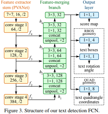
Finally, the network allows two types of outputs rotated bounding boxes: either a standard bounding box with a rotation angle (2X2+1 parameters) or “quadrangle” which is merely a rotated bounding box with coordinates of all vertices.
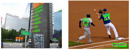
If real life results will be as in the above images, recognizing the texts will not take much of an effort. However, real life results are not perfect.
CRNN
Convolutional-recurrent neural network, is an article from 2015, which suggest a hybrid (or tribrid?) end to end architecture, that is intended to capture words, in a three step approach.
The idea goes as follows: the first level is a standard fully convolutional network. The last layer of the net is defined as feature layer, and divided into “feature columns”. See in the image below how every such feature column is intended to represent a certain section in the text.

Afterwards, the feature columns are fed into a deep-bidirectional LSTM which outputs a sequence, and is intended for finding relations between the characters.
Finally, the third part is a transcription layer. Its goal is to take the messy character sequence, in which some characters are redundant and others are blank, and use probabilistic method to unify and make sense out of it.
This method is called CTC loss, and can be read about here. This layer can be used with/without predefined lexicon, which may facilitate predictions of words.
This paper reaches high (>95%) rates of accuracy with fixed text lexicon, and varying rates of success without it.
STN-net/SEE
SEE — Semi-Supervised End-to-End Scene Text Recognition, is a work by Christian Bartzi. He and his colleagues apply a truly end to end strategy to detect and recognize text. They use very weak supervision (which they refer to as semi-supervision, in a different meaning than usual ). as they train the network with only text annotation (without bounding boxes). This allows them use more data, but makes their training procedure quite challenging, and they discuss different tricks to make it work, e.g not training on images with more than two lines of text (at least at the first stages of training).
The paper has an earlier version which is called STN OCR. In the final paper the researchers have refined their methods and presentation, and additionally they’ve put more emphasis on the generality of their approach on the account of high quality of the results.
The name STN-OCR hints on the strategy, of using spatial transformer(=STN, no relation to the recent google transformer).
They train two concatenated networks in which the first network, the transformer, learns a transformation on the image to output an easier sub-image to interpret.
Then, another feed forward network with LSTM on top (hmm… seems like we’ve seen it before) to recognize the text.
The researches emphasize here the importance of using resnet(they use it twice) since it provides “strong” propagation to the early layers. however this practice quite accepted nowadays.
Either way, this is an interesting approach to try.
3. Standard deep learning approach
As the header implies, after detecting the “words” we can apply standard deep learning detection approaches, such as SSD, YOLO and Mask RCNN. I’m not going to elaborate too much on theses approaches since there is a plethora of info online.
I must say this is currently my favorite approach, since what I like in deep learning is the “end to end” philosophy, where you apply a strong model which with some tuning will solve almost every problem. In the next section of this post we will see how it actually works.
However, SSD and other detection models are challenged when it comes to dense, similar classes, as reviewed here. I find it a bit ironic since in fact, deep learning models find it much more difficult to recognize digits and letters than to recognize much more challenging and elaborate objects such as dogs, cats or humans. They tend no to reach the desired accuracy, and therefore, specialized approaches thrive.
Practical Example
So after all the talking, it’s time to get our hands dirty, and try some modelling ourselves. We will try the tackle SVHN task. The SVHN data contains three different data-sets: train, test and extra. The differences are not 100% clear, however the extra data-set which is the biggest (with ~500K samples) includes images that are somehow easier to recognize. So for the sake of this take we will use it.
To prepare for the task, do the following:
- You’ll need a basic GPU machine with Tensorflow≥1.4 and Keras≥2
- Clone the SSD_Keras project from here.
- Download the pre-trained SSD300 model on coco data-set from here.
- Clone this project’s repo from here..
- Download the extra.tar.gz file, which contains the extra images of SVHN data-set.
- Update all relevant paths in json_config.json in this project repo.
To efficiently follow the process, you should read the below instruction along with running the ssd_OCR.ipynb notebook from the project’s repo.
And… You are ready to start!
Step 1: parse the data
Like it or not, but there is no “golden” format for data representation in detection tasks. Some well known formats are: coco, via, pascal, xml. And there are more. For instance, the SVHN data-set is annotated with the obscure .mat format. Fortunately for us, this gist provides a slick read_process_h5 script to convert the .mat file to standard json, and you should go one step ahead and convert it further to pascal format, like so:
def json_to_pascal(json, filename): #filename is the .mat file
    # convert json to pascal and save as csv
    pascal_list = []
    for i in json:
        for j in range(len(i['labels'])):
            pascal_list.append({'fname': i['filename']
            ,'xmin': int(i['left'][j]), 'xmax': int(i['left'][j]+i['width'][j])
            ,'ymin': int(i['top'][j]),  'ymax': int(i['top'][j]+i['height'][j])
            ,'class_id': int(i['labels'][j])})
    df_pascal = pd.DataFrame(pascal_list,dtype='str')
    df_pascal.to_csv(filename,index=False)p = read_process_h5(file_path)json_to_pascal(p, data_folder+'pascal.csv')
Now we should have a pascal.csv file that is much more standard and will allow us to progress. If the conversion is to slow, you should take note that we don’t need t all the data samples. ~10K will be enough.
Step 2: look at the data
Before starting the modeling process, you should better do some exploration of the data. I only provide a quick function for sanity test, but I recommend you to do some further analysis:
def viz_random_image(df):
    file = np.random.choice(df.fname)
    im = skimage.io.imread(data_folder+file)
    annots =  df[df.fname==file].iterrows()    plt.figure(figsize=(6,6))
    plt.imshow(im)    current_axis = plt.gca()    for box in annots:
        label = box[1]['class_id']
        current_axis.add_patch(plt.Rectangle(
            (box[1]['xmin'], box[1]['ymin']), box[1]['xmax']-box[1]['xmin'],
            box[1]['ymax']-box[1]['ymin'], color='blue', fill=False, linewidth=2))
        current_axis.text(box[1]['xmin'], box[1]['ymin'], label, size='x-large', color='white', bbox={'facecolor':'blue', 'alpha':1.0})
        plt.show()
viz_random_image(df)
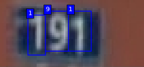
For the following steps, I provide a utils_ssd.py in the repo that facilitates the training, weight loading etc. Some of the code is taken from the SSD_Keras repo, which is also used extensively.
Step 3: choosing strategy
As previously discussed, we have many possible approaches for this problem. In this tutorial I’ll take standard deep learning detection approach, and will use the SSD detection model. We will use the SSD kerasimplementation from here. This is a nice Implementation by PierreLuigi. Although it has less GitHub stars than the rykov8 implementation, it seems more updated, and is easier to integrate. This is a very important thing to notice when you choose which project are you going to use. Other good choices will be the YOLO model, and the Mask RCNN.
Step 4: Load and train the SSD model
Some definitions
To use the repo, you’ll need to verify you have the SSD_keras repo, and fill in the paths in the json_config.json file, to allow the notebook finding the paths.
Start with importing:
import os
import sys
import skimage.io
import scipy
import jsonwith open('json_config.json') as f:     json_conf = json.load(f)ROOT_DIR = os.path.abspath(json_conf['ssd_folder']) # add here mask RCNN path
sys.path.append(ROOT_DIR)

import cv2
from utils_ssd import *
import pandas as pd
from PIL import Image

from matplotlib import pyplot as plt

%matplotlib inline
%load_ext autoreload
% autoreload 2
and some more definitions:
task = 'svhn'labels_path = f'{data_folder}pascal.csv'input_format = ['class_id','image_name','xmax','xmin','ymax','ymin' ]

df = pd.read_csv(labels_path)
Model configurations:
class SVHN_Config(Config):
    batch_size = 8

    dataset_folder = data_folder
    task = task

    labels_path = labels_path

    input_format = input_format

conf=SVHN_Config()

resize = Resize(height=conf.img_height, width=conf.img_width)
trans = [resize]
Define the model, load weights
As in most of deep learning cases, we won’t start training from scratch, but we’ll load pre-trained weights. In this case, we’ll load the weights of SSD model, trained on COCO data-set, which has 80 classes. Clearly our task has only 10 classes, therefore we will reconstruct the top layer to have the right number of outputs, after our loading the weights. We do it in the init_weights function. A side note: the right number of outputs in this case is 44: 4 for each class (bounding box coordinates) and another 4 for the background/none class.
learner = SSD_finetune(conf)
learner.get_data(create_subset=True)

weights_destination_path=learner.init_weights()

learner.get_model(mode='training', weights_path = weights_destination_path)
model = learner.model
learner.get_input_encoder()
ssd_input_encoder = learner.ssd_input_encoder

# Training schedule definitions
adam = Adam(lr=0.0002, beta_1=0.9, beta_2=0.999, epsilon=1e-08, decay=0.0)
ssd_loss = SSDLoss(neg_pos_ratio=3, n_neg_min=0, alpha=1.0)
model.compile(optimizer=adam, loss=ssd_loss.compute_loss)
Define data loaders
train_annotation_file=f'{conf.dataset_folder}train_pascal.csv'
val_annotation_file=f'{conf.dataset_folder}val_pascal.csv'
subset_annotation_file=f'{conf.dataset_folder}small_pascal.csv'batch_size=4
ret_5_elements={'original_images','processed_images','processed_labels','filenames','inverse_transform'}train_generator = learner.get_generator(batch_size, trans=trans, anot_file=train_annotation_file,
                  encoder=ssd_input_encoder)val_generator = learner.get_generator(batch_size,trans=trans, anot_file=val_annotation_file,
                 returns={'processed_images','encoded_labels'}, encoder=ssd_input_encoder,val=True)
5. Training the model
Now that the model is ready, we’ll set some last training related definitions, and start training
learner.init_training()history = learner.train(train_generator, val_generator, steps=100,epochs=80)
As a bonus, I’ve included the training_plot callback in the training script to visualize a random image after every epoch. For example, here is a snapshot of predictions after sixth epoch:
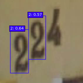
The SSD_Keras repo handles saving the model after almost each epoch , so you can load later the models simply by changing the weights_destination_path line to equal the path
weights_destination_path = <path>
If you followed my instructions, you should be able to train the model. The ssd_keras provides some more features, e.g data augmentations, different loaders, and evaluator. I’ve reached >80 mAP after short training.
How high did you achieve?
Summary
In this post, we discussed different challenges and approaches in the OCR field. As many problems in deep learning/computer vision, it has much more to it than seems at first. We have seen many sub tasks of it, and some different approaches to solve it, neither currently serves as a silver bullet. From the other hand, we’ve seen it is not very hard to reach preliminary results, without too much of hassle.
Hope you’ve enjoyed!

